Hands-on jaxparrow with Duacs data

The aim of this notebook is to illustrate how jaxparrow can be employed to derive geostrophic and cyclogeostrophic currents on a C-grid from Sea Surface Height (SSH) observations. The demo focuses on the Alboran Sea, a highly energetic area of the Mediterranean Sea (Ioannou et al. 2019).

We use the European Seas Gridded L4 Sea Surface Heights And Derived Variables Reprocessed dataset (description, reference). This product provides daily average of SSH, and geostrophic currents, on a rectilinear A-grid, with a spatial resolution of 1/8°.

We need to install some dependencies first:

!pip install ipympl matplotlib cartopy
!pip install copernicusmarine jaxparrow jaxtyping numpy xarray

%reload_ext autoreload
%autoreload 2

Accessing Duacs data

Copernicus Marine datasets can be accessed through the Copernicus Marine Toolbox API.

import copernicusmarine as cm

The API allows to download subsets of the datasets by restricting the spatial and temporal domains, and the variables.

import numpy as np

spatial_extent = (-5.3538, -1.1883, 35.0707, 36.8415)  # spatial extent (lon0, lon1, lat0, lat1) of the Alboran Sea
temporal_slice = (np.datetime64("2019-01-01T00:00:00"), np.datetime64("2019-12-31T23:59:59"))  # we look at the 2019 data for our demo
variables = ["adt", "ugos", "vgos"]  # we retrieve SSH and geostrophic currents (for comparison) data

dataset_options = {
    "dataset_id": "cmems_obs-sl_eur_phy-ssh_my_allsat-l4-duacs-0.125deg_P1D",
    "variables": variables,
    "minimum_longitude": spatial_extent[0],
    "maximum_longitude": spatial_extent[1],
    "minimum_latitude": spatial_extent[2],
    "maximum_latitude": spatial_extent[3],
    "start_datetime": temporal_slice[0],
    "end_datetime": temporal_slice[1]
}
duacs_ds = cm.open_dataset(**dataset_options)

Visualisation

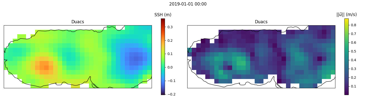
Lets visualise how the SSH, and the magnitude of the geostrophic currents, evolve over the time period.

duacs_ds = duacs_ds.assign(uvgos=np.sqrt(duacs_ds.ugos ** 2 + duacs_ds.vgos ** 2))

import matplotlib.pyplot as plt

from duacs_visualisation import AnimatedSSHCurrent
%matplotlib widget

anim = AnimatedSSHCurrent(duacs_ds, ("adt", "uvgos"), ("Duacs", "Duacs"))
plt.show()

Geostrophic currents using jaxparrow

jaxparrow uses C-grids, following NEMO convention. U, V, and F points are automatically derived from the T points.

import jax.numpy as jnp  # we manipulate jax.Array

lat_t = jnp.ones((duacs_ds.latitude.size, duacs_ds.longitude.size)) * duacs_ds.latitude.data.reshape(-1, 1)
lon_t = jnp.ones((duacs_ds.latitude.size, duacs_ds.longitude.size)) * duacs_ds.longitude.data

The spatial domain covers sea and land, we derive tbe mask to exclude the land parts of the domain from the adt invalid values.

adt_t = jnp.asarray(duacs_ds.adt.data)
mask = ~(jnp.isfinite(adt_t))

And we compute the geostrophic currents using the geostrophy function.

Rather than looping over our time indices, we can vectorise the geostrophy function over the time axis and compute the geostrophic currents at every time point using the vectorise version.

import jax
import jaxparrow as jpw

vmap_geostrophy = jax.vmap(jpw.geostrophy, in_axes=(0, None, None, 0), out_axes=(0, 0, None, None, None, None))

ug_jpw_u, vg_jpw_v, lat_u, lon_u, lat_v, lon_v = vmap_geostrophy(adt_t, lat_t, lon_t, mask)

To visualise the results, we compute the magnitude of the velocity.

from jaxparrow.tools.kinematics import magnitude

uvg_jpw_t = jax.vmap(magnitude, in_axes=(0, 0))(ug_jpw_u, vg_jpw_v)

We store everything in an xarray Dataset.

import xarray as xr

gos_jpw_ds = xr.Dataset(
    {
        "adt": (["time", "latitude", "longitude"], adt_t),
        "ug": (["time", "latitude_u", "longitude_u"], ug_jpw_u),
        "vg": (["time", "latitude_v", "longitude_v"], vg_jpw_v),
        "uvg": (["time", "latitude", "longitude"], uvg_jpw_t)
    },
    coords={
        "time": duacs_ds.time,
        "latitude": duacs_ds.latitude, "longitude": duacs_ds.longitude,
        "latitude_u": np.unique(lat_u).astype(np.float32), "longitude_u": np.unique(lon_u).astype(np.float32),
        "latitude_v": np.unique(lat_v).astype(np.float32), "longitude_v": np.unique(lon_v).astype(np.float32)
    }
)

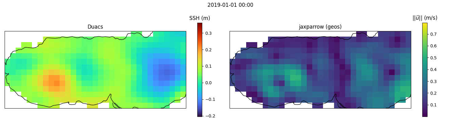
Visualisation

anim = AnimatedSSHCurrent(gos_jpw_ds, ("adt", "uvg"), ("Duacs", "jaxparrow (geos)"))
plt.show()

Geostrophic inter-comparison

For sanity check we can compare the two geostrophic reconstructions.

from duacs_visualisation import AnimatedCurrents

gos_ds = xr.Dataset(
    {
        "uvg": (["time", "latitude", "longitude"], duacs_ds.uvgos.data),
        "uvg_jpw": (["time", "latitude", "longitude"], uvg_jpw_t)
    },
    coords={
        "time": duacs_ds.time,
        "latitude": duacs_ds.latitude, "longitude": duacs_ds.longitude
    }
)

anim = AnimatedCurrents(gos_ds, ("uvg", "uvg_jpw"), ("Duacs", "jaxparrow"))
plt.show()

Cyclogeostrophic currents using jaxparrow

Now, lets see the results of the variational inversion of the cyclogeostrophic currents.

vmap_cyclogeostrophy = jax.vmap(jpw.cyclogeostrophy, in_axes=(0, None, None, 0), out_axes=(0, 0, None, None, None, None))

uc_jpw_u, vc_jpw_v, lat_u, lon_u, lat_v, lon_v = vmap_cyclogeostrophy(adt_t, lat_t, lon_t, mask)

uvc_jpw_t = jax.vmap(magnitude, in_axes=(0, 0))(uc_jpw_u, vc_jpw_v)

/Users/bertrava/projects/jaxparrow/venv/lib/python3.9/site-packages/matplotlib/animation.py:892: UserWarning: Animation was deleted without rendering anything. This is most likely not intended. To prevent deletion, assign the Animation to a variable, e.g. `anim`, that exists until you output the Animation using `plt.show()` or `anim.save()`.
  warnings.warn(

cgos_jpw_ds = xr.Dataset(
    {
        "adt": (["time", "latitude", "longitude"], adt_t),
        "uc": (["time", "latitude_u", "longitude_u"], uc_jpw_u),
        "vc": (["time", "latitude_v", "longitude_v"], vc_jpw_v),
        "uvc": (["time", "latitude", "longitude"], uvc_jpw_t)
    },
    coords={
        "time": duacs_ds.time,
        "latitude": duacs_ds.latitude, "longitude": duacs_ds.longitude,
        "latitude_u": np.unique(lat_u).astype(np.float32), "longitude_u": np.unique(lon_u).astype(np.float32),
        "latitude_v": np.unique(lat_v).astype(np.float32), "longitude_v": np.unique(lon_v).astype(np.float32)
    }
)

Visualisation

anim = AnimatedSSHCurrent(cgos_jpw_ds, ("adt", "uvc"), ("Duacs", "jaxparrow (cyclogeos)"))
plt.show()

Comparison with geostrophy

jpw_ds = xr.Dataset(
    {
        "uvg": (["time", "latitude", "longitude"], uvg_jpw_t),
        "uvc": (["time", "latitude", "longitude"], uvc_jpw_t)
    },
    coords={
        "time": duacs_ds.time,
        "latitude": duacs_ds.latitude, "longitude": duacs_ds.longitude
    }
)

anim = AnimatedCurrents(jpw_ds, ("uvg", "uvc"), ("geostrophy", "cyclogeostrophy"))
plt.show()