import os

from cartopy import crs as ccrs
import jax.numpy as jnp
import matplotlib.pyplot as plt
import numpy as np
import numpy.ma as ma
import optax
import xarray as xr

from jaxparrow import cyclogeostrophy, geostrophy
from jaxparrow.tools import geometry, kinematics, operators

%reload_ext autoreload
%autoreload 2

# utility functions

vmin = -4
vmax = -vmin
dpi_ref = 100
full_width_px = 1600


def get_figsize(width_ratio, wh_ratio=1):
    fig_width = full_width_px / dpi_ref * width_ratio
    fig_height = fig_width / wh_ratio
    return fig_width, fig_height

Method validation using the eNATL60 run

Input data

In this example, we use NEMO model outputs (SSH and velocities), stored in several netCDF files. Measurements are located on a C-grid.

Data can be downloaded here, and the files extracted to the data folder. The next cell does this for you, assuming wget and tar are available.

!wget -P data https://ige-meom-opendap.univ-grenoble-alpes.fr/thredds/fileServer/meomopendap/extract/MEOM/jaxparrow/alboransea.tar.gz
!tar -xzf data/alboransea.tar.gz -C data
!rm data/alboransea.tar.gz

data_dir = "data"
name_mask = "mask_alboransea.nc"
name_coord = "coordinates_alboransea.nc"
name_ssh = "alboransea_sossheig.nc"
name_u = "alboransea_sozocrtx.nc"
name_v = "alboransea_somecrty.nc"

ds_coord = xr.open_dataset(os.path.join(data_dir, name_coord))
lat_t = jnp.copy(ds_coord.nav_lat.values)
lon_t = jnp.copy(ds_coord.nav_lon.values)

ds_mask = xr.open_dataset(os.path.join(data_dir, name_mask))
mask = jnp.copy(ds_mask.tmask[0,0].values)

ds_ssh = xr.open_dataset(os.path.join(data_dir, name_ssh))
ssh = jnp.copy(ds_ssh.sossheig[0].values)

ds_u = xr.open_dataset(os.path.join(data_dir, name_u))
uvel = jnp.copy(ds_u.sozocrtx[0].values)

ds_v = xr.open_dataset(os.path.join(data_dir, name_v))
vvel = jnp.copy(ds_v.somecrty[0].values)

We use a mask array to restrict the domain to the marine area.

mask = 1 - mask

jaxparrow only needs the coordinates of the T points of the grid (lat and lon here). The corresponding U and V coordinates are derived automatically using NEMO convention see, as in our example.

lat_u, lon_u, lat_v, lon_v = geometry.compute_uv_grids(lat_t, lon_t)

Visualising SSH and currents

# compute some characteristics
norm_vorticity_t = kinematics.normalized_relative_vorticity(
    uvel, vvel, lat_u, lon_u, lat_v, lon_v, mask, interpolate=True
)
magnitude = ma.masked_array(kinematics.magnitude(uvel, vvel, interpolate=True), mask)

mmin = np.nanmin(magnitude)
mmax = np.nanmax(magnitude)

# interpolate to the center of the cells
uvel_t = operators.interpolation(uvel, axis=1, padding="left")
vvel_t = operators.interpolation(vvel, axis=0, padding="left")

_, (ax1, ax2, ax3) = plt.subplots(1, 3, figsize=get_figsize(1, 20/3),
                                  subplot_kw={"projection": ccrs.PlateCarree()})

ax1.set_title("Sea Surface Height")
im = ax1.pcolormesh(lon_t, lat_t, ma.masked_array(ssh, mask),
                    cmap="turbo", shading="auto",
                    transform=ccrs.PlateCarree())
clb1 = plt.colorbar(im, ax=ax1)
clb1.ax.set_title("SSH (m)")

ax2.set_title("Current velocity")
im = ax2.pcolormesh(lon_t, lat_t, magnitude,
                    shading="auto",
                    transform=ccrs.PlateCarree())
ax2.quiver(lon_t[::5, ::5], lat_t[::5, ::5],
           ma.masked_array(uvel_t, mask)[::5, ::5], ma.masked_array(vvel_t, mask)[::5, ::5],
           color="k")
clb2 = plt.colorbar(im, ax=ax2)
clb2.ax.set_title("$\\vert\\vert \\vec{u} \\vert\\vert$ (m/s)")

ax3.set_title("Current normalized vorticity")
im = ax3.pcolormesh(lon_t, lat_t, norm_vorticity_t,
                    cmap="RdBu_r", shading="auto",
                    vmin=vmin, vmax=vmax,
                    transform=ccrs.PlateCarree())
clb3 = plt.colorbar(im, ax=ax3)
clb3.ax.set_title("$\\xi / f$")

plt.show()

png

Geostrophic balance

We estimate the geostrophic velocities using the geostrophy function, given the SSH, the coordinates of the T points, and an optional mask. The function can also returns the the U and V coordinates of the velocity U and V components (they are the same as the one computed earlier for illustration, so we use return_grids=False).

u_geos, v_geos = geostrophy(ssh, lat_t, lon_t, mask, return_grids=False)

norm_vorticity_geos_t = kinematics.normalized_relative_vorticity(u_geos, v_geos, lat_u, lon_u, lat_v, lon_v, mask, interpolate=True)

Comparison to NEMO’s velocities

fig, axs = plt.subplots(2, 2, figsize=get_figsize(2/3, 12.66/6),
                        subplot_kw={"projection": ccrs.PlateCarree()})

axs[0, 0].set_title("NEMO data")
_ = axs[0, 0].pcolormesh(lon_t, lat_t, norm_vorticity_t,
                         cmap="RdBu_r", shading="auto",
                         vmin=vmin, vmax=vmax,
                         transform=ccrs.PlateCarree())

axs[0, 1].set_title("Geostrophy")
im1 = axs[0, 1].pcolormesh(lon_t, lat_t, norm_vorticity_geos_t,
                           cmap="RdBu_r", shading="auto",
                           vmin=vmin, vmax=vmax,
                           transform=ccrs.PlateCarree())

_ = axs[1, 0].pcolormesh(lon_t, lat_t, magnitude,
                         shading="auto",
                         vmin=mmin, vmax=mmax,
                         transform=ccrs.PlateCarree())

im2 = axs[1, 1].pcolormesh(lon_t, lat_t, kinematics.magnitude(u_geos, v_geos, interpolate=True),
                           shading="auto",
                           vmin=mmin, vmax=mmax,
                           transform=ccrs.PlateCarree())

fig.tight_layout()
fig.subplots_adjust(right=0.89, wspace=0.01)

cbar_ax1 = fig.add_axes([0.9, 0.51, 0.01, 0.38])
_ = fig.colorbar(im1, cax=cbar_ax1)
cbar_ax1.set_title("$\\xi / f$")

cbar_ax2 = fig.add_axes([0.9, 0.05, 0.01, 0.38])
_ = fig.colorbar(im2, cax=cbar_ax2)
cbar_ax2.set_title("$\\vert\\vert \\vec{u} \\vert\\vert$")

plt.show()

png

Cyclogeostrophic balance

Variational method

Cyclogeostrophic velocities are computed via the cyclogeostrophy function, using geostrophic velocities (here, the ones we previously computed), spatial steps, and the coriolis factors.

The optimizer can be specified as a string (assuming it refers to an optax common optimizers): optim = "sgd" for example. Or designed using a more refined strategy:

lr_scheduler = optax.exponential_decay(1e-2, 200, .5)  # decrease the learning rate
optim = optax.sgd(learning_rate=lr_scheduler)  # basic SGD works nicely
optim = optax.chain(optax.clip(1), optim)  # prevent updates from exploding

As for the geostrophy, the cyclogeostrophy function can return the U and V points in addition to the velocity components. If specifying return_geos=True, the function also returns the geostrophic velocity. Lastly, it is possible to get the evaluation of the cyclogeostrophic imbalance at each iteration by passing return_losses=True.

u_var, v_var, losses_var = cyclogeostrophy(ssh, lat_t, lon_t, mask, optim=optim, return_geos=False, return_grids=False, return_losses=True)

norm_vorticity_var_t = kinematics.normalized_relative_vorticity(u_var, v_var, lat_u, lon_u, lat_v, lon_v, mask, interpolate=True)

Comparison to NEMO’s velocities

fig, axs = plt.subplots(2, 2, figsize=get_figsize(1, 20/6),
                        subplot_kw={"projection": ccrs.PlateCarree()})

axs[0, 0].set_title("NEMO data")
_ = axs[0, 0].pcolormesh(lon_t, lat_t, norm_vorticity_t, cmap="RdBu_r", shading="auto",
                         vmin=vmin, vmax=vmax,
                         transform=ccrs.PlateCarree())

axs[0, 1].set_title("Variational cyclogeostrophy")
im1 = axs[0, 1].pcolormesh(lon_t, lat_t, norm_vorticity_var_t, cmap="RdBu_r", shading="auto",
                          vmin=vmin, vmax=vmax,
                          transform=ccrs.PlateCarree())

_ = axs[1, 0].pcolormesh(lon_t, lat_t, magnitude,
                         shading="auto",
                         vmin=mmin, vmax=mmax,
                         transform=ccrs.PlateCarree())

im2 = axs[1, 1].pcolormesh(lon_t, lat_t, kinematics.magnitude(u_var, v_var, interpolate=True),
                           shading="auto",
                           vmin=mmin, vmax=mmax,
                           transform=ccrs.PlateCarree())

fig.tight_layout()
fig.subplots_adjust(right=0.64, wspace=0.01)

cbar_ax1 = fig.add_axes([0.65, 0.51, 0.01, 0.38])
_ = fig.colorbar(im1, cax=cbar_ax1)
cbar_ax1.set_title("$\\xi / f$")

cbar_ax2 = fig.add_axes([0.65, 0.05, 0.01, 0.38])
_ = fig.colorbar(im2, cax=cbar_ax2)
cbar_ax2.set_title("$\\vert\\vert \\vec{u} \\vert\\vert$")

ax3 = fig.add_axes([0.73, 0.3, 0.27, 0.4])
ax3.set_title("Cyclogeostrophic disequilibrium - $J(\\vec{u}_c^{(n)})$")
ax3.set_xlabel("step")
ax3.set_ylabel("disequilibrium")
ax3.plot(losses_var)

plt.show()

png

Iterative method

We use the same function, but with the argument method="iterative".

u_iterative, v_iterative, losses_it = cyclogeostrophy(ssh, lat_t, lon_t, mask, method="iterative",
                                                      return_geos=False, return_grids=False, return_losses=True)

norm_vorticity_iterative_t = kinematics.normalized_relative_vorticity(u_iterative, v_iterative, lat_u, lon_u, lat_v, lon_v, mask, interpolate=True)

Comparison to NEMO’s velocities

fig, axs = plt.subplots(2, 2, figsize=get_figsize(1, 20/6),
                        subplot_kw={"projection": ccrs.PlateCarree()})

axs[0, 0].set_title("NEMO data")
_ = axs[0, 0].pcolormesh(lon_t, lat_t, norm_vorticity_t, cmap="RdBu_r", shading="auto",
                         vmin=vmin, vmax=vmax,
                         transform=ccrs.PlateCarree())

axs[0, 1].set_title("Iterative cyclogeostrophy")
im1 = axs[0, 1].pcolormesh(lon_t, lat_t, norm_vorticity_iterative_t, cmap="RdBu_r", shading="auto",
                           vmin=vmin, vmax=vmax,
                           transform=ccrs.PlateCarree())

_ = axs[1, 0].pcolormesh(lon_t, lat_t, magnitude,
                         shading="auto",
                         vmin=mmin, vmax=mmax,
                         transform=ccrs.PlateCarree())

im2 = axs[1, 1].pcolormesh(lon_t, lat_t, kinematics.magnitude(u_iterative, v_iterative, interpolate=True),
                           shading="auto",
                           vmin=mmin, vmax=mmax,
                           transform=ccrs.PlateCarree())

fig.tight_layout()
fig.subplots_adjust(right=0.64, wspace=0.01)

cbar_ax1 = fig.add_axes([0.65, 0.51, 0.01, 0.38])
_ = fig.colorbar(im1, cax=cbar_ax1)
cbar_ax1.set_title("$\\xi / f$")

cbar_ax2 = fig.add_axes([0.65, 0.05, 0.01, 0.38])
_ = fig.colorbar(im2, cax=cbar_ax2)
cbar_ax2.set_title("$\\vert\\vert \\vec{u} \\vert\\vert$")

ax3 = fig.add_axes([0.73, 0.3, 0.27, 0.4])
ax3.set_title("Cyclogeostrophic disequilibrium - $J(\\vec{u}_c^{(n)})$")
ax3.set_xlabel("step")
ax3.set_ylabel("disequilibrium")
ax3.plot(losses_it)

plt.show()

png

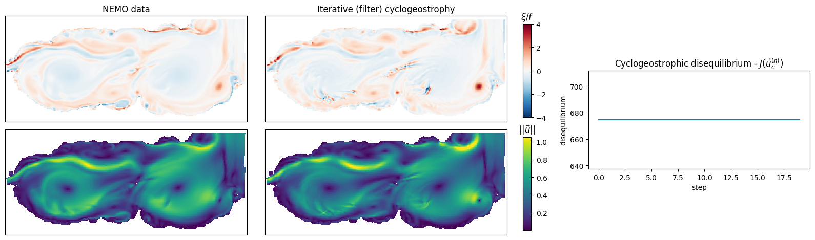
Iterative method, with filter

We use the same function, but with the arguments method="iterative", and use_res_filter=True.

u_it_filter, v_it_filter, losses_it_filter = cyclogeostrophy(ssh, lat_t, lon_t, mask, method="iterative", use_res_filter=True,
                                                             return_geos=False, return_grids=False, return_losses=True)

norm_vorticity_it_filter_t = kinematics.normalized_relative_vorticity(u_it_filter, v_it_filter, lat_u, lon_u, lat_v, lon_v, mask, interpolate=True)

Comparison to NEMO’s currents

fig, axs = plt.subplots(2, 2, figsize=get_figsize(1, 20/6),
                        subplot_kw={"projection": ccrs.PlateCarree()})

axs[0, 0].set_title("NEMO data")
_ = axs[0, 0].pcolormesh(lon_t, lat_t, norm_vorticity_t, cmap="RdBu_r", shading="auto",
                         vmin=vmin, vmax=vmax,
                         transform=ccrs.PlateCarree())

axs[0, 1].set_title("Iterative (filter) cyclogeostrophy")
im1 = axs[0, 1].pcolormesh(lon_t, lat_t, norm_vorticity_it_filter_t, cmap="RdBu_r", shading="auto",
                           vmin=vmin, vmax=vmax,
                           transform=ccrs.PlateCarree())

_ = axs[1, 0].pcolormesh(lon_t, lat_t, magnitude,
                         shading="auto",
                         vmin=mmin, vmax=mmax,
                         transform=ccrs.PlateCarree())

im2 = axs[1, 1].pcolormesh(lon_t, lat_t, kinematics.magnitude(u_it_filter, v_it_filter, interpolate=True),
                           shading="auto",
                           vmin=mmin, vmax=mmax,
                           transform=ccrs.PlateCarree())

fig.tight_layout()
fig.subplots_adjust(right=0.64, wspace=0.01)

cbar_ax1 = fig.add_axes([0.65, 0.51, 0.01, 0.38])
_ = fig.colorbar(im1, cax=cbar_ax1)
cbar_ax1.set_title("$\\xi / f$")

cbar_ax2 = fig.add_axes([0.65, 0.05, 0.01, 0.38])
_ = fig.colorbar(im2, cax=cbar_ax2)
cbar_ax2.set_title("$\\vert\\vert \\vec{u} \\vert\\vert$")

ax3 = fig.add_axes([0.73, 0.3, 0.27, 0.4])
ax3.set_title("Cyclogeostrophic disequilibrium - $J(\\vec{u}_c^{(n)})$")
ax3.set_xlabel("step")
ax3.set_ylabel("disequilibrium")
ax3.plot(losses_it_filter)

plt.show()

png

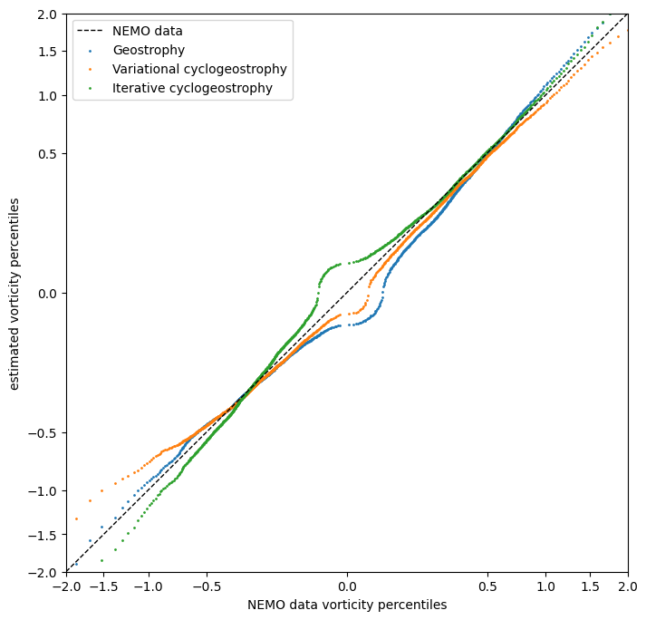
Overall quantitative comparison

percentiles = np.linspace(0, 1, 1000)
vorticity_percentile = np.quantile(norm_vorticity_t[~np.isnan(norm_vorticity_t)], percentiles)
vorticity_percentile_geos = np.quantile(norm_vorticity_geos_t[~np.isnan(norm_vorticity_geos_t)], percentiles)
vorticity_percentile_var = np.quantile(norm_vorticity_var_t[~np.isnan(norm_vorticity_var_t)], percentiles)
vorticity_percentile_iterative = np.quantile(norm_vorticity_iterative_t[~np.isnan(norm_vorticity_iterative_t)], percentiles)

fig = plt.figure(figsize=get_figsize(.5))
ax = fig.add_subplot(1, 1, 1)
ax.axline(xy1=(vorticity_percentile.min(), vorticity_percentile.min()),
          xy2=(vorticity_percentile.max(), vorticity_percentile.max()),
          linestyle="dashed", linewidth=1, color="black", label="NEMO data")
ax.scatter(vorticity_percentile, vorticity_percentile_geos,
           s=1, label="Geostrophy")
ax.scatter(vorticity_percentile, vorticity_percentile_var,
           s=1, label="Variational cyclogeostrophy")
ax.scatter(vorticity_percentile, vorticity_percentile_iterative,
           s=1, label="Iterative cyclogeostrophy")
ax.legend()
ax.set_xlabel("NEMO data vorticity percentiles")
ax.set_ylabel("estimated vorticity percentiles")
ax.set_xscale('function', functions=(lambda x: np.sign(x) * np.sqrt(np.abs(x)),
                                     lambda x: np.sign(x) * x**2))
ax.set_yscale('function', functions=(lambda x: np.sign(x) * np.sqrt(np.abs(x)),
                                     lambda x: np.sign(x) * x**2))
ax.set_xlim((-2, 2))
ax.set_ylim((-2, 2))

plt.show()

png